Spot the blob on the job
- nicoaguila93
- Dec 27, 2020
- 2 min read
On December 9's session, objects were labeled and measured as blobs and connected components
Blob Detection
Blobs are objects of interest in a given image. In order to determine blobs, they must be defined as bright objects in a dark background to ensure that algorithms will be able to properly detect them. Three methods were discussed to detect blobs:
Laplacian of Gaussian (LoG) - Laplacian of a Gaussian smoothed image
Difference of Gaussian (DoG) - Difference of Two Gaussian smoothed images
Determinant of Hessian (DoH) - Maximum value in the matrix of the Determinant of Hessian
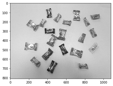
Original Reference Image on the left and a Binarized Reference Image on the right


LoG, DoG, and DoH Blob Detection algorithms, respectively.

Based on the nature of the reference image, LoG would be the best suited algorithm for this case as it properly identifies the shape of the candy wrappers, unlike the other two where circles are dominantly seen that are sometimes separate in nature despite being enclosed in one candy wrapper.
Connected Components
Despite LoG appearing accurate in blob detection for our reference image, all three algorithms try to identify the blobs by marking them as circular objects. Since not all objects are circular, and that there are even objects of irregular shape, connected components in an image can be considered as objects of interest instead. However, connected components rely heavily on the image structure, which is why image cleaning is a must, which can be done using morphological operations.
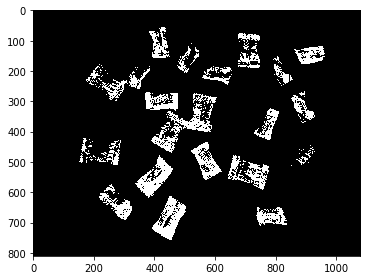
Binarized reference image on the left and cleaned via multiple erosion and dilation on the right

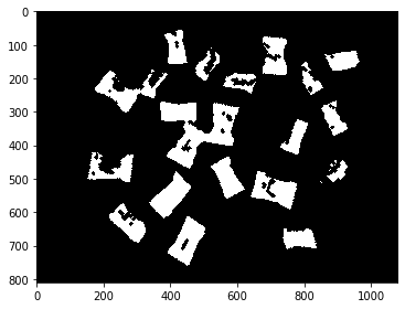
Once cleaned, mapping of the connected components are then done. With this, region properties of the connected components can be identified.
Connected components mapped with their corresponding region properties

The connected components are mapped as pixels wrapped again in matrices, just like how filtering and morphological operations to their job, by identifying objects in which to apply their operations on.
Given the coordinates on the image, we can determine the connected components via the regionprop module in Python:
from skimage.measure import label, regionprops
label_im = label(im_cleaned) #im_cleaned is the cleaned binarized #reference image
props=regionprops(label_im)
#Example:
props[5].centroid
(168.8494856524093, 496.53329723876556)By using the centroid parameter of regionprop, we can determine the coordinates of the centroids of some of the connected components identified by the algorithm.


Comments